Early Software Estimation
Early estimates of schedule, resourcing and cost are generally required for most software projects. Despite it’s criticality to successful project completion, software estimation is most often done poorly, often arbitrarily. How can this be improved for early project estimation?
Despite many years of research into the topic, many (probably most) project exceed their budget and schedule. According to Capers Jones [1], data shows that many projects whose size is about 1000 function points are delayed or cancelled (38%). For those projects around 10K FP most projects are delayed or cancelled (72%). See the full table below for the probability of selected outcomes.
Size (FP) |
Early |
On Time |
Delayed |
Cancelled |
1 |
14.68 |
83.16 |
1.92 |
0.25 |
10 |
11.08 |
81.25 |
5.67 |
2.00 |
100 |
6.06 |
74.77 |
11.83 |
7.33 |
1,000 |
1.24 |
60.76 |
17.67 |
20.33 |
10,000 |
0.14 |
28.03 |
23.83 |
48.00 |
100,000 |
0.00 |
13.67 |
21.33 |
65.00 |
Average |
5.53 |
56.94 |
13.71 |
23.82 |
To understand this table, you will need to know a little about function point conversion into your language of choice. LOC to FP conversion tables have been published [2] [3] [4], however using backfiring to produce function point counts is known to not be accurate. We will accept this restriction for the purpose of this post. I have published selected values from [4] below.
Language |
LOC/FP Mean |
C |
128 |
C++ |
53 |
Smalltalk |
21 |
SQL |
12 |
To make calculations simple, assume the Java/C++ is 50 LOC/FP. Therefore a 50K LOC Java program is about 1000 FP and about a 60% chance of on time delivery.
The most common form of software estimation is still expert based, usually from similar projects from memory or by intuition, often with little evidence to backup the validity of the estimate. Expert based opinion is:
-
often wrong
-
hard to validate
-
lessons learned are usually not learned
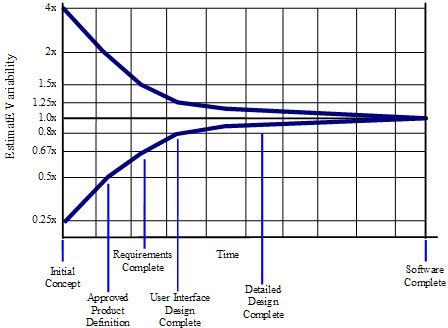
Assuming an initial estimate is need early in the project lifecycle, what data can we use to give an estimate that is not required to be precise due to the cone of uncertainty
Sizing
Initial software size can be performed by category or analogy. See my previous post on Fast Software Sizing
Effort and Schedule
Although software estimation is a complex activity based on many factors (the COCOMO model lists more than 20) various rules of thumb can be used early in the project. Jones' rule of thumb for staff size is the size in FP divided by 150 is the number of personnel for the application. For our example of 1000 FP, this gives ~6.7 people.
staff = FP size / 150
The schedule is approximated by:
schedule (months) = FP ^ 0.4
Although 0.4 is the average, web based software uses the exponent of 0.35. For our example, using 0.35, the schedule is then ~11.2 months.
Staff effort is then calculated by multiply the schedule by the staff size. For our example this gives 75 staff months. If we make an assumption that staff cost $72K/year, then the project will cost $450K. Of course this excludes typical overhead costs and other factors. The productivity on this project would then be 1000 FP / 75 staff months = 13.3 FP / month. For comparison, the U.S. average was 13.6 for 1000 FP applications [5].
A word of warning that the staffing in this example is reasonably different than table 3-22 in [5] where the average staff for a web based application of 1000 FP is 3.9 and schedule is 10 months in table 3-25. Initially I suspected this would primarily be due to the lower staff size required for web based applciations. However, table 3-30 in [5] lists productivity in web based applications to be 25.6 FP/month, almost double the productivity figure of 13.3 given above. If we use this higher productivity figure then the cost of a 1000 FP web based application is 1000 / 25.6 = 39.1 staff months. The full table of productivity for various application types of various sizes is given below.
Application Type |
100 |
1K |
10K |
100K |
Average |
End-user |
52.60 |
na |
na |
na |
52.60 |
Web |
47.30 |
25.60 |
12.00 |
na |
28.30 |
MIS |
21.00 |
16.40 |
4.65 |
2.70 |
11.19 |
U.S. outsource |
23.00 |
17.20 |
4.90 |
3.20 |
12.08 |
Offshore outsource |
19.00 |
15.80 |
4.70 |
3.00 |
10.63 |
Commercial |
11.00 |
9.30 |
4.60 |
4.00 |
7.23 |
Systems |
9.00 |
6.90 |
5.10 |
4.15 |
6.29 |
Military |
5.60 |
4.80 |
3.80 |
2.10 |
4.08 |
Average |
23.56 |
13.71 |
5.68 |
3.19 |
11.54 |
All estimation should be done using various techniques, ideally converging and reinforcing the appropriateness of each other, negating bias from any particular technique.
Conclusion
Despite producing fairly inaccurate results, early software sizing is possible and useful. This is a nice supplement to formal estimation models and expert opinion for software estimates early in the lifecycle.
Bibliography
-
[1] Jones, Estimating Software Costs: Bringing Realism to Estimating, 2007.
-
[2] QSM Function Point Languages Table, http://www.qsm.com/resources/function-point-languages-table.
-
[3] Mayes Consulting Function Point Conversion, http://softwareestimator.com/IndustryData2.htm.
-
[5] Jones, Applied Software Measurement: Global Analysis of Productivity and Quality, 2008.
-
[7] Molokken, A Review of Surveys on Software Effort Estimation.
-
[8] The Data & Analysis Center for Software (DACS), Fast Function Points Overview.
-
[9] McConnell, Software Estimation: Demystifying the Black Art, 2006.


